Landscape of ODE Solvers in R

Solving ordinary differential equations (ODEs) is a common task in many fields, including systems biology, pharmacometrics, and engineering. The R ecosystem offers a collection of tools for this purpose: from lightweight numerical solvers to full modeling frameworks.

This article provides a practical overview of ODE solvers in R, with a focus on helping users navigate the ecosystem and choose appropriate tools.

All packages here was tested with simple examples and the code was published in the GitHub repository.

What is included

We include tools that:

• Provide an API for R
• Support solving general ODE systems
• Are mentioned in literature, documentation, or community discussions

We intentionally exclude:

• Deprecated or archived packages (e.g., RxODE)
• Thin wrappers around other frameworks without original solvers or formats (e.g., nlmixr2)
• Small helper packages
• Highly specialized tools limited to narrow domains

Some tools included in this review go beyond ODE solving and provide additional capabilities such as parameter estimation or simulation workflows. We include them for completeness, without going into those advanced features.

Overview table

Type

• Pure R solvers: Numerical algorithms implemented directly in R. These are easy to inspect and flexible, but typically slower due to interpreter overhead.
• Compiled solvers: Implemented in C/C++/Fortran or wrapping established libraries (e.g., ODEPACK). These provide significantly better performance and are the default choice for most applications.
• External runtime interfaces: Packages that delegate computation to external ecosystems such as Julia or Python. These act as bridges rather than standalone solvers.

Engine / Algorithms

• Engine refers to the underlying numerical implementation used by the package. This can be:

  • a well-known external library (e.g., ODEPACK),
  • a custom compiled implementation,
  • or an external runtime (e.g., Julia),
  • another R package.

• Algorithms lists the available numerical methods (e.g., LSODA, Runge–Kutta, Radau).
  Some packages expose multiple algorithms, while others are limited to a specific class.

Model format

ODE models can be defined in different ways: as R functions, domain-specific languages (DSL), structured APIs, or even external code.

The key distinction affecting performance is how the model is executed:

• Interpreted execution: The model is defined as an R function and evaluated during each solver step.
• Compiled execution: The model is translated into compiled code before simulation, avoiding interpreter overhead and improving performance.

Stiff

Indicates whether the solver can handle stiff systems.

Stiffness arises when a system contains processes evolving on very different time scales. Solvers that support stiffness typically use implicit methods or adaptive switching (e.g., LSODA).

DAE / DDE

Support for these features is solver-dependent and often requires specific algorithms.

• DAE (Differential-Algebraic Equations): Systems that include algebraic constraints in addition to differential equations.
• DDE (Delay Differential Equations): Systems where derivatives depend on past states.

Time events / Conditional events

These features are important for modeling real-world systems with discontinuities.

• Time events: Discrete changes applied at predefined time points (e.g., dosing events).
• Conditional events: Events triggered when a condition is met during simulation (e.g., threshold crossing).

CRAN downloads

Total number of downloads in 2025, reflecting usage statistics.

Repository and test cases

To ensure practical consistency, packages were tested on two simple ODE models. The full code for all packages is available in the companion GitHub repository.

We are providing here the code in mrgsolve format for two examples: a pharmacokinetic model with non-linear elimination, and the Robertson problem, which is a classic stiff ODE system.

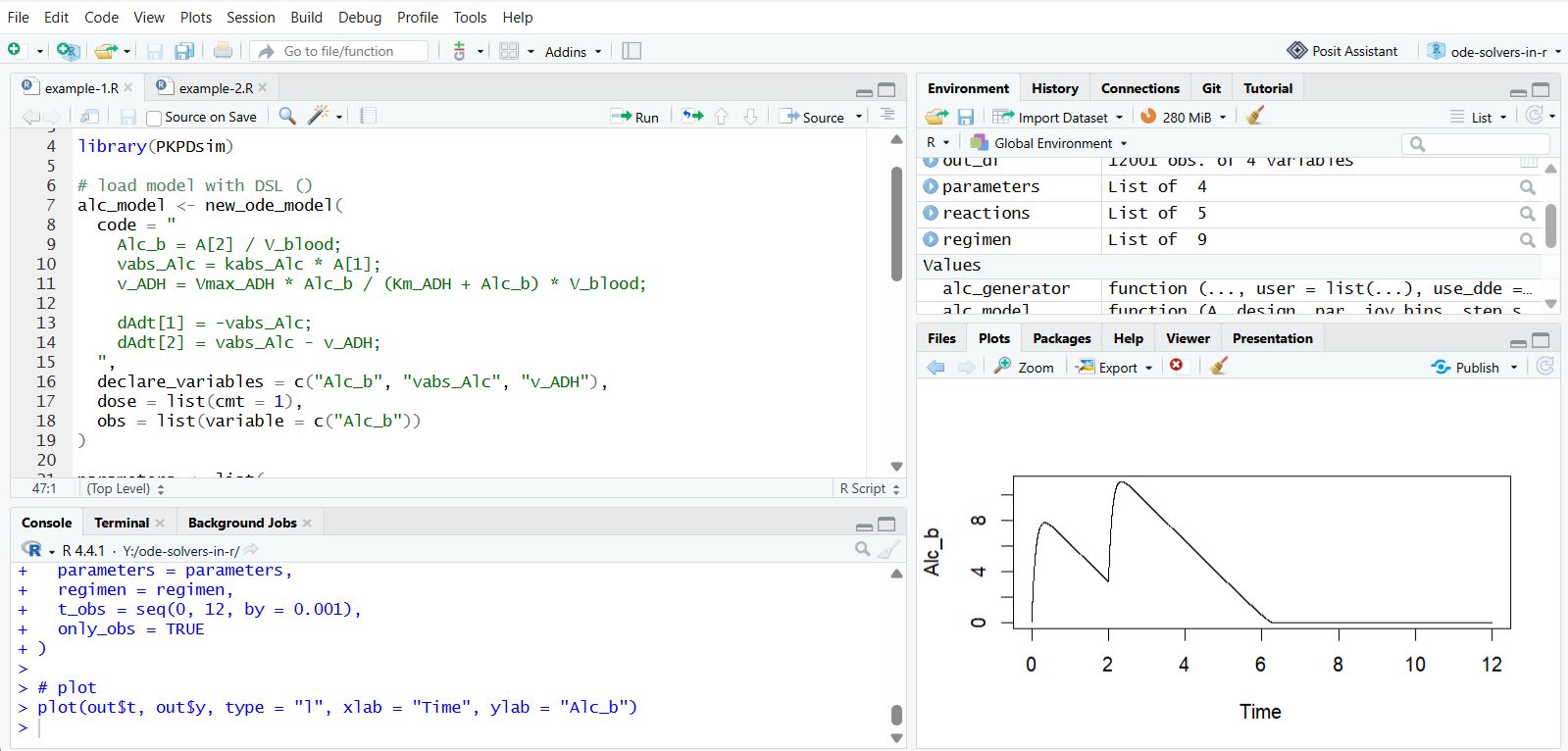
Example 1: Pharmacokinetic model with non-linear elimination

library(mrgsolve)
library(magrittr)

# load model as DLS (C++ like)
mod <- mcode("pk_model", '
$PARAM
kabs_Alc = 10.0
Vmax_ADH = 3
Km_ADH = 0.1
V_blood = 5.5

$CMT
Alc_g Alc_b_amt

$ODE
double Alc_b = Alc_b_amt / V_blood;
double vabs_Alc = kabs_Alc * Alc_g;
double v_ADH = Vmax_ADH * Alc_b / (Km_ADH + Alc_b) * V_blood;

dxdt_Alc_g = -vabs_Alc;
dxdt_Alc_b_amt = vabs_Alc - v_ADH;

$TABLE
capture Alc_b;
')

# time event
ev1 <- ev(time = 2, amt = 50, cmt = "Alc_g")

# solve
out <- mod %>%
  init(Alc_g = 50, Alc_b_amt = 0) %>%
  ev(ev1) %>%
  mrgsim(start = 0, end = 12, delta = 0.001)

plot(out)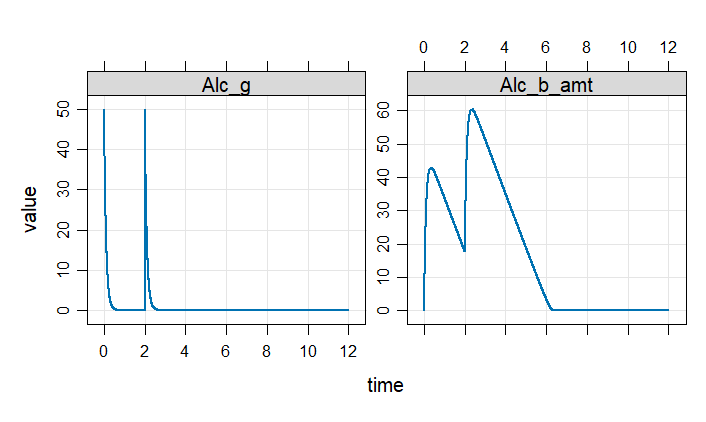

Example 2: Robertson problem stiff ODE

library(mrgsolve)
library(magrittr)

# load model as DLS (C++ like)
mod <- mcode("rob_model", '
$CMT
A B C

$ODE
dxdt_A = -0.04 * A + 1e4 * B * C;
dxdt_B =  0.04 * A - 1e4 * B * C - 3e7 * pow(B, 2);
dxdt_C =  3e7 * pow(B, 2);
')

# solve
out <- mod %>%
  init(A = 1, B = 0, C = 0) %>%
  mrgsim(start = 0, end = 1, delta = 1e-2)

plot(out)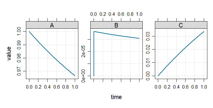

Author's notes

The goal of this review was to provide a maximally complete and objective overview of tools for solving ODEs in R. The packages included in this survey differ significantly in their purpose and functionality: from simple numerical solvers to full-featured frameworks and specialized domain-specific tools. They are presented here on equal footing, without going into detailed feature comparisons.

Many aspects - such as computational performance, numerical accuracy, and advanced functionality - are intentionally not covered in this article.

The table includes popularity metrics in the form of download counts. However, these numbers do not reflect the actual capabilities of the packages. Downloads may include one-time installations for educational purposes, CI/CD workflows, or other non-analytical uses. Therefore, they should not be considered a deciding factor when choosing a tool, but rather as a rough indicator of visibility within the community.

Below is a subjective selection of packages that I would recommend paying attention to.

General-purpose solution: deSolve

deSolve is a robust and well-established package with broad functionality and support for multiple numerical methods. It provides advanced capabilities such as handling stiffness, DAEs, DDEs, and events, while maintaining good computational performance through compiled solvers and model interfaces. It also offers flexible ways to define models.

With a large user base and extensive documentation, it is a reliable default choice.

I would recommend it as a general-purpose tool for most ODE tasks in R. If you are new to ODE modeling in R, starting with deSolve is a safe and practical choice before exploring more specialized tools.

Domain-specific tool: rxode2

rxode2 is a powerful tool designed for pharmacokinetics and pharmacodynamics (PK/PD).

Together with the nlmixr2 toolkit, it extends beyond ODE solving to include parameter estimation from data and efficient Monte Carlo simulations in parallel and distributed environments.

If your work is related to PK/PD modeling, this can be an excellent choice.

Underappreciated tool: dMod

dMod provides a powerful framework for dynamic modeling, parameter estimation, and identifiability analysis.

It combines symbolic model definition with efficient numerical solvers and supports gradient-based optimization workflows. While it has a steeper learning curve compared to simpler solvers, it offers a high level of flexibility and is particularly useful for more advanced modeling tasks.

Despite its capabilities, it appears to be less widely used, making it an interesting but often overlooked option.

Bridge to high-performance: diffeqr

diffeqr provides an interface to the Julia-based DifferentialEquations.jl ecosystem, exposing a large collection of state-of-the-art solvers directly in R.

Rather than implementing its own numerical methods, it delegates computation to Julia, allowing access to advanced algorithms, GPU acceleration, and high-performance execution that are often beyond native R tools.